library(biogeonet)
Philosophy
In Cazelles1, we basically expand the classical Theory of Island Biogeography2 to include ecological interactions and a link to the environmental niche. To do so we:
- simulated ecological networks of 10 species using the niche model3
- link the simulated ecological interactions to extinction probability
- link an arbitrary environmental gradient to the colonization probability
- use all the steps above to create the transition matrix of a Markov chain (from any of the \(2^{10}\) communities to any other) and then solve it to obtain the presence absence of all communities.
Niche model
To simulate I use the niche model that I implemented in nicheModel(). The first parameters, nbsp, determines the number of species:
nicheModel(nbsp = 5, .2, 1)
#>            [,1]       [,2]        [,3]        [,4]      [,5]
#> [1,]  0.0000000  0.0000000  0.00000000  0.33236422 0.0000000
#> [2,]  0.0000000  0.0000000  0.00000000  0.03608205 0.0000000
#> [3,]  0.0000000  0.0000000  0.00000000  0.77903683 0.0000000
#> [4,] -0.2483893 -0.2615522 -0.03363379 -0.56977655 0.7670426
#> [5,]  0.0000000  0.0000000  0.00000000 -0.08233662 0.0000000
nicheModel(nbsp = 10, .2, 1)
#>              [,1]       [,2]       [,3]        [,4]       [,5]       [,6]
#>  [1,]  0.00000000  0.0000000  0.3841360  0.85394965  0.0000000  0.0000000
#>  [2,]  0.00000000 -0.3750247 -0.9981889  0.95745936  0.0000000  0.0000000
#>  [3,] -0.98501505  0.8154719  0.0000000  0.66046801  0.0000000  0.0000000
#>  [4,] -0.02846291 -0.5160620 -0.4495050 -0.92402186  0.0000000  0.4072649
#>  [5,]  0.00000000  0.0000000  0.0000000  0.00000000  0.0000000  0.2341506
#>  [6,]  0.00000000  0.0000000  0.0000000 -0.62204806 -0.2942034 -0.3762614
#>  [7,]  0.00000000 -0.4999713 -0.5694014 -0.01884913 -0.6807970  0.6601791
#>  [8,]  0.00000000 -0.7282874 -0.1698769  0.00000000  0.0000000  0.0000000
#>  [9,] -0.76358026  0.0000000  0.0000000  0.00000000  0.0000000  0.0000000
#> [10,]  0.00000000 -0.3374719 -0.3382163 -0.35345944 -0.5736737  0.0000000
#>               [,7]      [,8]      [,9]     [,10]
#>  [1,]  0.000000000 0.0000000 0.3642837 0.0000000
#>  [2,]  0.344138852 0.8830474 0.0000000 0.8076427
#>  [3,]  0.007748912 0.5956353 0.0000000 0.4507875
#>  [4,]  0.347627673 0.0000000 0.0000000 0.6339386
#>  [5,]  0.786232939 0.0000000 0.0000000 0.2205929
#>  [6,] -0.382116071 0.0000000 0.0000000 0.0000000
#>  [7,]  0.000000000 0.0000000 0.0000000 0.0000000
#>  [8,]  0.000000000 0.0000000 0.0000000 0.0000000
#>  [9,]  0.000000000 0.0000000 0.0000000 0.0000000
#> [10,]  0.000000000 0.0000000 0.0000000 0.0000000
The second parameter controls the expected connectance.
nicheModel(5, connec = .1, 1)
#>             [,1]       [,2] [,3]      [,4] [,5]
#> [1,]  0.00000000  0.8851977    0 0.9109430    0
#> [2,] -0.06858638  0.0000000    0 0.1818991    0
#> [3,]  0.00000000  0.0000000    0 0.0000000    0
#> [4,] -0.91030452 -0.4129825    0 0.0000000    0
#> [5,]  0.00000000  0.0000000    0 0.0000000    0
nicheModel(5, connec = .4, 1)
#>            [,1]        [,2]        [,3]       [,4]      [,5]
#> [1,] -0.9841690  0.00000000  0.29242813  0.0000000 0.0000000
#> [2,]  0.0000000  0.00000000  0.82954198  0.3879820 0.2239297
#> [3,] -0.5189022 -0.08568547  0.00000000  0.8029444 0.0000000
#> [4,]  0.0000000 -0.44476858 -0.02897205 -0.6111635 0.0000000
#> [5,]  0.0000000 -0.82795797  0.00000000  0.0000000 0.0000000
The last parameter, mode, affects the sign structure of the output matrix (not included in the original publication of the niche model):
# mode 1 + and -, refered as "predation" in Cazelles (2016)
nicheModel(5, .2, mode = 1)
#>            [,1]       [,2]       [,3] [,4]     [,5]
#> [1,]  0.0000000  0.8030849  0.0000000    0 0.000000
#> [2,] -0.8579318  0.0000000  0.1610954    0 0.336101
#> [3,]  0.0000000 -0.2457675 -0.7525627    0 0.000000
#> [4,]  0.0000000  0.0000000  0.0000000    0 0.000000
#> [5,]  0.0000000 -0.4672883  0.0000000    0 0.000000
# mode 2, only -, refered as "competition" in Cazelles (2016)
nicheModel(5, .2, mode = 2)
#>            [,1]       [,2]        [,3]        [,4]       [,5]
#> [1,]  0.0000000 -0.8275084 -0.28216915 -0.08436808 -0.1292878
#> [2,] -0.5868197 -0.2568651 -0.02139296 -0.09211540 -0.9332288
#> [3,] -0.3046849 -0.3417499  0.00000000  0.00000000 -0.4632092
#> [4,] -0.5982661 -0.1033734  0.00000000  0.00000000 -0.6710231
#> [5,] -0.6106307 -0.2024269 -0.67715417 -0.72855328 -0.8842671
# mode 2, only +, refered as "mutualism" in Cazelles (2016)
nicheModel(5, .2, mode = 3)
#>           [,1]     [,2]      [,3] [,4] [,5]
#> [1,] 0.9061011 0.000000 0.1060589    0    0
#> [2,] 0.0000000 0.000000 0.2712583    0    0
#> [3,] 0.8293471 0.403457 0.2538694    0    0
#> [4,] 0.0000000 0.000000 0.0000000    0    0
#> [5,] 0.0000000 0.000000 0.0000000    0    0
See ?nicheModel for further details.
Colonization
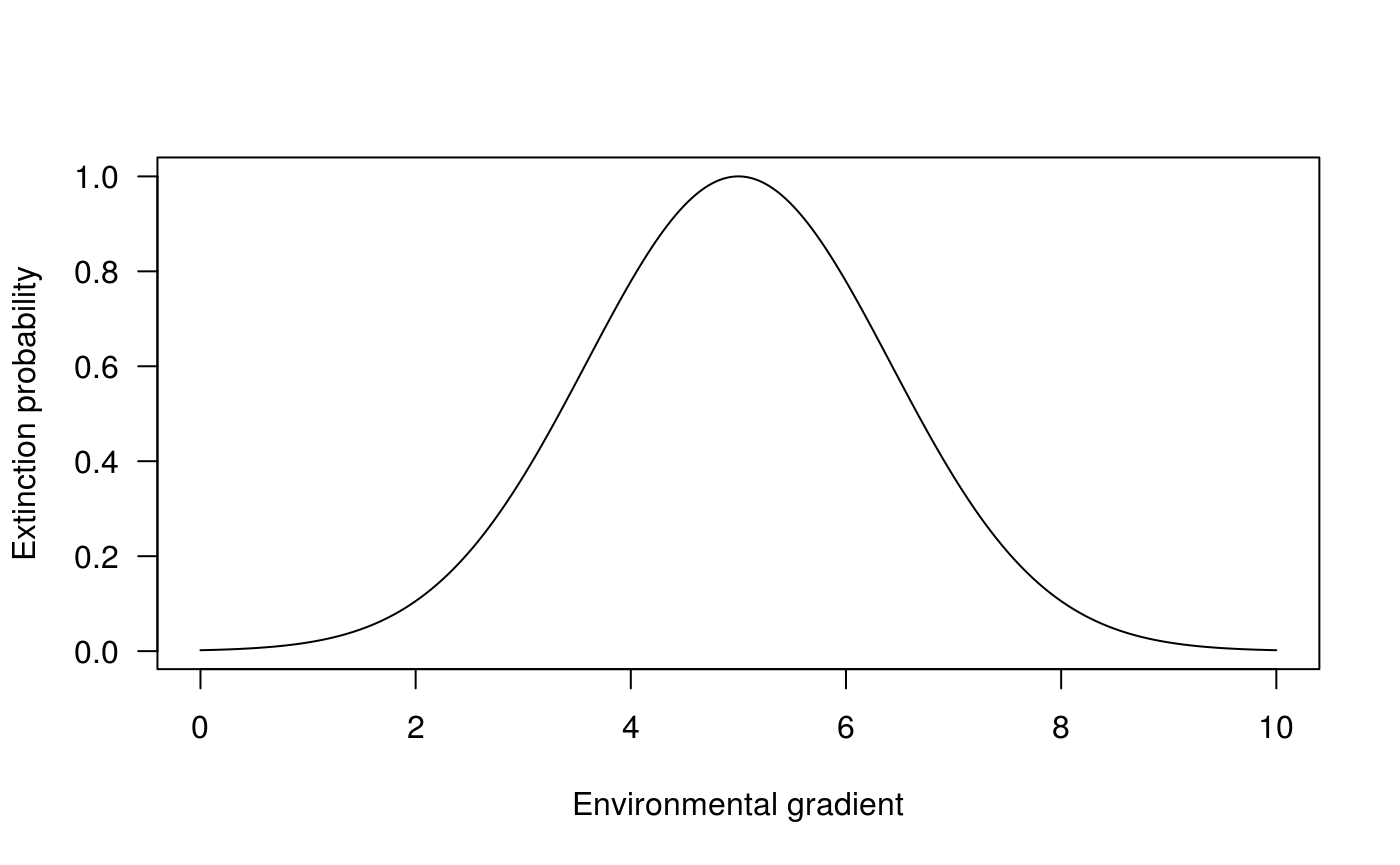
The colonisation probability is a bell-shaped function (see ?colonization for details).
seqx <- seq(0, 10, .01)
vc_colo <- sapply(seqx, FUN = colonization, 1, 5, 2)
plot(seqx, vc_colo, type="l", las = 1, ylab = "Extinction probability",
  xlab = "Environmental gradient")
Extinction
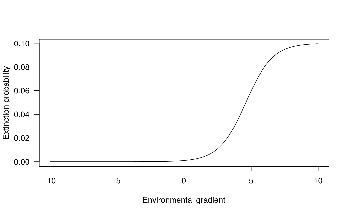
The extinction probability is basically a flexible logistic function (see ?extinction for details)
seqx <- seq(-10, 10, .01)
vc_exti <- sapply(seqx, FUN = extinction, 1e-3, 1e-2, 1e2, -1)
plot(seqx, vc_exti, type="l", las = 1, ylab = "Extinction probability",
  xlab = "Environmental gradient")
Building Markov chain and deriving its equilibrium
For a specific vector of colonisation (1 value per species), a specific ecological networks (use to derive extinction probabilities), we can build the transition matrix of a Markov chain with buildMarkov(). So far, it builds the matrix of a continuous-time Markov chain](https://en.wikipedia.org/wiki/Markov_chain#Continuous-time_Markov_chain) ans so probabilities described above should actually be rates.
# number of species
nbsp <- 4
# network
web <- nicheModel(nbsp, .2, mode = 1)
# colonisation vector
colo <- 10^runif(nbsp, -7, -3)
#
mat <- buildMarkov(nbsp, colo, web, 1e-5, 1e-3, 1e3, -1)
mat
#> $markov
#>                [,1]          [,2]          [,3]          [,4]          [,5]
#>  [1,] -3.619764e-04  1.000000e-05  7.930139e-06  0.000000e+00  4.208889e-06
#>  [2,]  5.804130e-06 -3.661723e-04  0.000000e+00  7.123548e-06  0.000000e+00
#>  [3,]  3.240423e-04  0.000000e+00 -4.586422e-05  2.383297e-05  0.000000e+00
#>  [4,]  0.000000e+00  3.240423e-04  5.804130e-06 -6.308648e-05  0.000000e+00
#>  [5,]  1.780241e-05  0.000000e+00  0.000000e+00  0.000000e+00 -3.483829e-04
#>  [6,]  0.000000e+00  1.780241e-05  0.000000e+00  0.000000e+00  5.804130e-06
#>  [7,]  0.000000e+00  0.000000e+00  1.780241e-05  0.000000e+00  3.240423e-04
#>  [8,]  0.000000e+00  0.000000e+00  0.000000e+00  1.780241e-05  0.000000e+00
#>  [9,]  1.432754e-05  0.000000e+00  0.000000e+00  0.000000e+00  0.000000e+00
#> [10,]  0.000000e+00  1.432754e-05  0.000000e+00  0.000000e+00  0.000000e+00
#> [11,]  0.000000e+00  0.000000e+00  1.432754e-05  0.000000e+00  0.000000e+00
#> [12,]  0.000000e+00  0.000000e+00  0.000000e+00  1.432754e-05  0.000000e+00
#> [13,]  0.000000e+00  0.000000e+00  0.000000e+00  0.000000e+00  1.432754e-05
#> [14,]  0.000000e+00  0.000000e+00  0.000000e+00  0.000000e+00  0.000000e+00
#> [15,]  0.000000e+00  0.000000e+00  0.000000e+00  0.000000e+00  0.000000e+00
#> [16,]  0.000000e+00  0.000000e+00  0.000000e+00  0.000000e+00  0.000000e+00
#>                [,6]          [,7]          [,8]          [,9]         [,10]
#>  [1,]  0.000000e+00  0.000000e+00  0.000000e+00  7.525700e-06  0.000000e+00
#>  [2,]  4.208889e-06  0.000000e+00  0.000000e+00  0.000000e+00  7.525700e-06
#>  [3,]  0.000000e+00  4.208889e-06  0.000000e+00  0.000000e+00  0.000000e+00
#>  [4,]  0.000000e+00  0.000000e+00  4.208889e-06  0.000000e+00  0.000000e+00
#>  [5,]  1.000000e-05  7.930139e-06  0.000000e+00  0.000000e+00  0.000000e+00
#>  [6,] -3.525788e-04  0.000000e+00  7.123548e-06  0.000000e+00  0.000000e+00
#>  [7,]  0.000000e+00 -3.227070e-05  2.383297e-05  0.000000e+00  0.000000e+00
#>  [8,]  3.240423e-04  5.804130e-06 -4.949296e-05  0.000000e+00  0.000000e+00
#>  [9,]  0.000000e+00  0.000000e+00  0.000000e+00 -3.551746e-04  1.000000e-05
#> [10,]  0.000000e+00  0.000000e+00  0.000000e+00  5.804130e-06 -3.593704e-04
#> [11,]  0.000000e+00  0.000000e+00  0.000000e+00  3.240423e-04  0.000000e+00
#> [12,]  0.000000e+00  0.000000e+00  0.000000e+00  0.000000e+00  3.240423e-04
#> [13,]  0.000000e+00  0.000000e+00  0.000000e+00  1.780241e-05  0.000000e+00
#> [14,]  1.432754e-05  0.000000e+00  0.000000e+00  0.000000e+00  1.780241e-05
#> [15,]  0.000000e+00  1.432754e-05  0.000000e+00  0.000000e+00  0.000000e+00
#> [16,]  0.000000e+00  0.000000e+00  1.432754e-05  0.000000e+00  0.000000e+00
#>               [,11]         [,12]         [,13]         [,14]         [,15]
#>  [1,]  0.000000e+00  0.000000e+00  0.000000e+00  0.000000e+00  0.000000e+00
#>  [2,]  0.000000e+00  0.000000e+00  0.000000e+00  0.000000e+00  0.000000e+00
#>  [3,]  7.525700e-06  0.000000e+00  0.000000e+00  0.000000e+00  0.000000e+00
#>  [4,]  0.000000e+00  7.525700e-06  0.000000e+00  0.000000e+00  0.000000e+00
#>  [5,]  0.000000e+00  0.000000e+00  5.097426e-06  0.000000e+00  0.000000e+00
#>  [6,]  0.000000e+00  0.000000e+00  0.000000e+00  5.097426e-06  0.000000e+00
#>  [7,]  0.000000e+00  0.000000e+00  0.000000e+00  0.000000e+00  5.097426e-06
#>  [8,]  0.000000e+00  0.000000e+00  0.000000e+00  0.000000e+00  0.000000e+00
#>  [9,]  7.930139e-06  0.000000e+00  7.301092e-06  0.000000e+00  0.000000e+00
#> [10,]  0.000000e+00  7.123548e-06  0.000000e+00  7.301092e-06  0.000000e+00
#> [11,] -3.906238e-05  2.383297e-05  0.000000e+00  0.000000e+00  7.301092e-06
#> [12,]  5.804130e-06 -5.628463e-05  0.000000e+00  0.000000e+00  0.000000e+00
#> [13,]  0.000000e+00  0.000000e+00 -3.422450e-04  1.000000e-05  7.930139e-06
#> [14,]  0.000000e+00  0.000000e+00  5.804130e-06 -3.464408e-04  0.000000e+00
#> [15,]  1.780241e-05  0.000000e+00  3.240423e-04  0.000000e+00 -2.613279e-05
#> [16,]  0.000000e+00  1.780241e-05  0.000000e+00  3.240423e-04  5.804130e-06
#>               [,16]
#>  [1,]  0.000000e+00
#>  [2,]  0.000000e+00
#>  [3,]  0.000000e+00
#>  [4,]  0.000000e+00
#>  [5,]  0.000000e+00
#>  [6,]  0.000000e+00
#>  [7,]  0.000000e+00
#>  [8,]  5.097426e-06
#>  [9,]  0.000000e+00
#> [10,]  0.000000e+00
#> [11,]  0.000000e+00
#> [12,]  7.301092e-06
#> [13,]  0.000000e+00
#> [14,]  7.123548e-06
#> [15,]  2.383297e-05
#> [16,] -4.335504e-05
#>
#> $speciesRichness
#>  [1] 0 1 1 2 1 2 2 3 1 2 2 3 2 3 3 4
#>
#> $speciesPresence
#>      [,1] [,2] [,3] [,4] [,5] [,6] [,7] [,8] [,9] [,10] [,11] [,12] [,13] [,14]
#> [1,]    0    1    0    1    0    1    0    1    0     1     0     1     0     1
#> [2,]    0    0    1    1    0    0    1    1    0     0     1     1     0     0
#> [3,]    0    0    0    0    1    1    1    1    0     0     0     0     1     1
#> [4,]    0    0    0    0    0    0    0    0    1     1     1     1     1     1
#>      [,15] [,16]
#> [1,]     0     1
#> [2,]     1     1
#> [3,]     1     1
#> [4,]     1     1
then solveMarkov() returns the probabilities at equilibrium for all communities:
sol <- solveMarkov(mat$markov, continuous = TRUE)
sol
#>  [1] 8.143621e-06 4.495148e-07 1.388899e-02 8.476522e-04 6.992460e-05
#>  [6] 3.859726e-06 1.192568e-01 7.278304e-03 5.635265e-05 3.110576e-06
#> [11] 9.610974e-02 5.865628e-03 4.178675e-04 2.306561e-05 7.126752e-01
#> [16] 4.349494e-02
This gives the probability at equilibrium (sensu MacArthur & Wilson 1967) for all of the \(2^{nbsp}\) community (here nbsp=4, so there are 16 potential communities).
# NB sum to one
sum(sol)
#> [1] 1
In order to compute the species richness, one simply needs to compute the expectation value of the random variable that associates to every state, its species richness, i.e.:
sum(sol * mat$speciesRichness)
#> [1] 2.7988
Similarly, one can compute the expected presence of all species
mat$speciesPresence %*% sol
#>            [,1]
#> [1,] 0.05751701
#> [2,] 0.99941723
#> [3,] 0.88321993
#> [4,] 0.85864590
Reproduce the study
In Cazelles et al. (2016), we basically solved tons of those for 10 species (1024 communities), for the 3 sign structure described above and under various scenarios of connectance and environmental conditions (so a bunch of for loops using the steps described above!).
Cazelles, K., Mouquet, N., Mouillot, D. & Gravel, D. 2016. On the integration of biotic interaction and environmental constraints at the biogeographical scale. Ecography. 39, 921–931. DOI: 10.1111/ecog.01714.↩︎
MacArthur, R. H. and Wilson, E. O. 1967. Theory of island biogeography. – Princeton Univ. Press. ISBN: 0691088365.↩︎
Williams, R. J. and Martinez, N. D. 2000. Simple rules yield complex food webs. – Nature 404: 180–183.DOI:10.1038/35004572.↩︎