Outline
- Introduction
- The
graphicspackage basis - Composition and multi-panel plotting
- Graphics automation and exporting
- Resources
- Exercises
Kevin Cazelles and Nicolas Casajus
Université du Québec à Rimouski
graphics package basisA picture is worth a thousand words

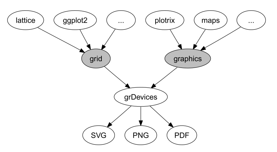
plot()boxplot(), barplot(), hist()lines(), points(), legend()ggplot2 is based on this packagegrid packagegrid packageand requires a long time to master it
See the QCBS workshop on ggplot2
graphics packagegraphics packageboxplot2)graphics packagepar() returns their valuespar() allows changing the valuesopar <- par()par(col='red')par(opar)opar <- par()par(col = 'red')par(opar)plot(), boxplot(), barplot(), hist(), etc.plot(), boxplot(), barplot(), hist(), etc.lines(), points(), axis(), legend(), etc.You only need to know one high-level plotting function:
plot()
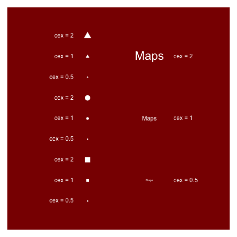
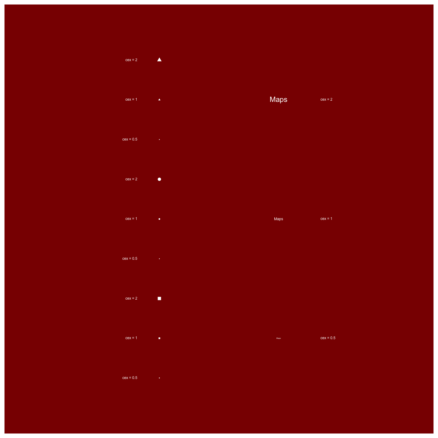
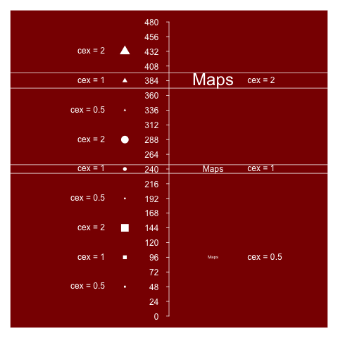
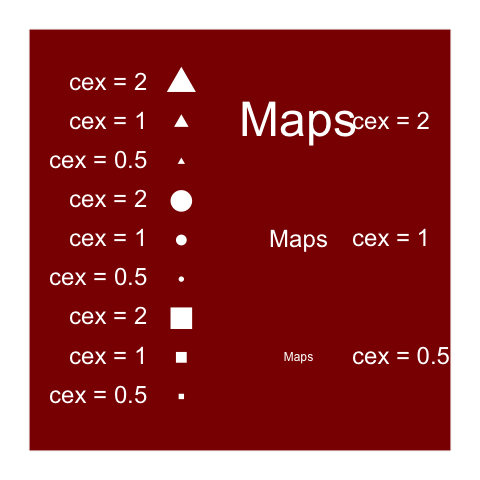
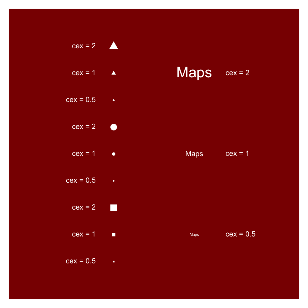
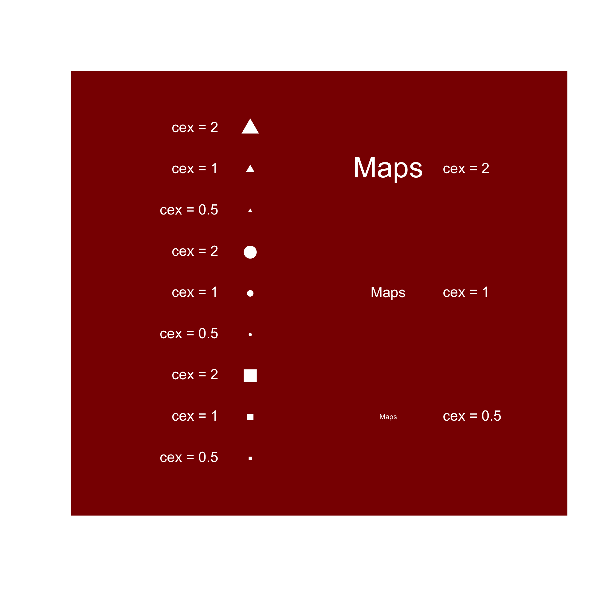
bty (default: 'o')ann (default: 'TRUE')xaxt (default: 's')yaxt (default: 's')axes=FALSE is the same as:bty='n'+xaxt='n'+yaxt='n'type (default: 'p')type (default: 'p')points() or axis()points()plot()cex, the sizecol, the colorpch, the symbolcol: the border color,bg: the background colorpch = 21 to 25points()lines()abline()segments()abline()abline() allows to draw horizontal and vertical lineslines() and points()lines() and points()lwd, the line widthcol, the line colorlty, the line typepolygon()rect()polygon()border, the border colorcol, the background colorlwd, the border widthrect() is appropriated when you want to add draw rectangletitle()text()cex, the sizecol, the colorfont, the font (bold, italic, etc.)family, the typefacesrt, the rotation anglepos, the position from coordinatestext() can't add text outside the plot areapar(xpd=TRUE)mtext()## Basic colors
palette()
## [1] "transparent" "darkred" "#505050" "#4E7BDB"
## and 657 others colors
colors()[1:10]
##  [1] "white"         "aliceblue"     "antiquewhite"  "antiquewhite1"
##  [5] "antiquewhite2" "antiquewhite3" "antiquewhite4" "aquamarine"
##  [9] "aquamarine1"   "aquamarine2"
rgb()red <- rgb(red = 1, green = 0, blue = 0)
yellow <- rgb(red = 1, green = 1, blue = 0)
gray1 <- rgb(red = 0.5, green = 0.5, blue = 0.5)
rgb()red <- rgb(red = 1, green = 0, blue = 0)
yellow <- rgb(red = 1, green = 1, blue = 0)
gray1 <- rgb(red = 0.5, green = 0.5, blue = 0.5)
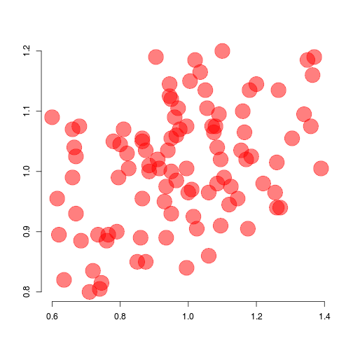
alpha argument controls for opacity (default = 1)## Transparent red
redp <- rgb(red = 1, green = 0, blue = 0,
alpha = .8)
## Empty plot
plot(x = dat$x, y = dat$y, ann = FALSE,
     bty = 'n', type = 'n')

## Transparent red
redp <- rgb(red = 1, green = 0, blue = 0,
            alpha = .5)

## Adding points
points(x = dat$x, y = dat$y, col = redp,
       pch = 19, cex = 4)
red    <- '#FF0000'
yellow <- '#FFFF00'
gray1  <- '#888888'
red    <- '#FF0000'
yellow <- '#FFFF00'
gray1  <- '#888888'
## Transparent red
redp <- '#FF000088'
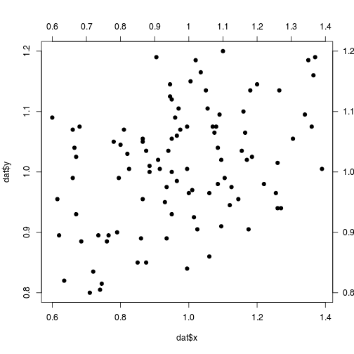
axis() allows to add axis## Empty plot
plot(x = dat$x, y = dat$y, pch = 19)
## Adding top-axis
axis(side = 3, at = seq(0.6, 1.4, by = 0.1),
labels = seq(0.6, 1.4, by = 0.1), las = 1)
## Adding right-axis
axis(side = 4, at = seq(0.8, 1.2, by = 0.1),
labels = format(seq(0.8, 1.2, by = 0.1)),
las = 2)
mar in the par()par(mar = c(4, 4, 4, 4))
mfrow and mfcol in par()par(mfrow=c(2,2))
or
par(mfcol=c(2,2))
mfrow and mfcol in par()split.screen()split.screen(c(1, 2))
split.screen(c(3, 1), screen = 2)
par()split.screen()mat_lay <- matrix(c(1,2,4,1,3,4),nrow=3)
layout(mat_lay)
mat_lay <- matrix(c(1,2,4,1,3,4), nrow=3)
layout(mat_lay)
##      [,1] [,2]
## [1,]    1    1
## [2,]    2    3
## [3,]    4    4
mat_lay <- matrix(c(0,2,2,1,3,3,1,4,0), nrow=3)
layout(mat_lay)
##      [,1] [,2] [,3]
## [1,]    0    1    1
## [2,]    2    3    4
## [3,]    2    3    0
mat_lay <- matrix(c(0,2,2,1,3,3,1,4,0),nrow=3)
layout(mat_lay, widths=c(.25,1,1))
mat_lay <- matrix(c(0,2,2,1,3,3,1,4,0),nrow=3)
layout(mat_lay, widths=c(.25,1,1),
  heights=c(.25,1,.25))
new=TRUEfig in par() plot(...)
new=TRUEfig in par()par(); plot(...)
par(new=TRUE, fig=c(0.5,1,0.5,1))
new=TRUEfig in par()par();add your embedded plot;
  plot(...)
  par(new=TRUE, fig=c(0.5,1,0.5,1))
plot(...)

options('device')
bmp(), jpeg(), png(), tiff()?jpeg
png(filename, width=480, height=480)
...
dev.off()
png(filename, width=1440, height=1440)
...
dev.off()
width=480 + height=480 = grid of 480x480px ;pointsize of plotted text = how many points your font will use (size of the text);res (in px per inch, ppi) links pixel and size;res determines how many pixels = 1pt;res=72 then one point will equal exactly one pixel.res=72 + width=480 + height=480 = 6.667x6.667in => 16.9*16.9cmres=300 + width=480 + height=480 = 1.6x1.6in => 4.06cmx4.06cmjpeg(filename, res=72,
pointsize=12, width=480, height=480)
...
dev.off()


png(filename, res=144)
...
dev.off()
png(filename, res=144,
  height=7, width=7, unit="in")
...
dev.off()
png(filename, res=288,
   height=7, width=7, unit="in")
...
dev.off()
png(filename, res=288,
  height=7, width=7, unit="in")
...
dev.off()
png(filename, res=288,
  height=2*7, width=7, unit="in")
...
dev.off()

pdf(fil, pointsize=12,
  height=2*7, width=7)
...
dev.off()
svg(filename, pointsize=12,
  height=2*7, width=7)
...
dev.off()

Reproduce the distribution of english letters made by David Taylor :
